Lesson 43 - EIGRP Fundamentals Part 1 - Overview

EIGRP is a Cisco Proprietary Routing Protocol. It is classified as an Advanced Distance Vector solution. EIGRP is a fast, modern and robust routing protocol offering features we expect to find in the routing protocol these days (as of the time of writing this tutorial).

EIGRP Characteristics

• Advanced Distance Vector Protocol - EIGRP routers, similarly to RIP, create the database in which only distance (how far) and direction (next-hop) are given. As a result of that, routers do not know the exact topology of the network. However, like in link-state algorithm, EIGRP routers are going to discover their neighbors using EIGRP Hello packets, form adjacency and exchange the routing databases reliably with their neighbors.
• Flexible Design - EIGRP does not use the concept of areas found in OSPF. It is less demanding in terms of the design allowing less experienced engineers implement it quickly. It supports summarization of prefixes on per interface-basis (unlike OSPF which does it on ABRs/ASBRs only). 
• Incremental Updates - Routing updates are not advertised periodically. They are exchanged reliably once (must beacknowledged). In stable network, only hello packets are transmitted between neighbors to maintain the relationship. In case of the topology change, the updates are sent to the routers that should receive it. The routers take into consideration how long it takes to send the reliable packet and get the response from a neighbor. Based on that, they determine how long they should wait to re-send the upate in case they did not get the acknowledgement. 
• VLSM Support - Although EIGRP is primary Distance Vector Protocol, it is a classless protocol which supports variable length subnet masking. In order to turn it on, you must use the 'no auto-summary' keyword in the routing process 'config-router'.
• Rapid Convergence - In case the EIGRP domain is designed with redundant connections and certain criteria are met (Feasibility Condition) a router can keep information about so called Feasible Successor(s) which are the second best path towards the destination (sort of a backup route). The difference between OSPF/RIP backup paths (second best routes) and EIGRP's feasible successor is that in the latter protocol, the traffic is redirected immediately without recomputing the routing table.
• Multicast - EIGRP uses multicast and unicast transmissions. Multicast address reserved for EIGRP is 224.0.0.10.
• 100% Loop Free - The Diffusing Update Algorithm (DUAL) which EIGRP uses, guarantees there are not going to be any loops formed which Distance Vector algorithms are susceptible to (thanks to the Feasibility Condition).
• Equal and Unequal Cost Load Balancing - EIGRP routers can utilize different paths with different metric performing a load balance. The router calculates the appropriate ratio regarding how many packet should be sent out the interface based on the difference in the metric value between these multiple paths available.
• Support for multiple layer 3 protocols - EIGRP can natively support IP,  IPX and Apple-Talk protocols (altough in today's IP world this is no longer a major advantage).

Based on my experience with EIGRP (personal opinion), the two major disadvantages of EIGRP are:

• It is very chatty if the network is not properly designed. Explanation of the design is beyond the scope of this tutorial.
• It is a Cisco proprietary routing protocol which means it won't work on routers from different vendors.

Terminology

EIGRP Databases

EIGRP creates three databases, similarly to OSPF:

• Neighbor Table - Lists all neighbors discovered with which it formed adjacency and exchanged routing information.
• Topology Table - Lists all the paths to all destinations learned. However, it shows only metric and the next-hop router and does not illustrate the real topology like OSPF LSDB.
• Routing Table - The best metric routes are going to be used to send the traffic. 

EIGRP Composite Metric
EIGRP calculates the metric using pretty complex formula which is beyond the scope of the CCNA tutorial. It is referred to as composite metric. EIGRP uses five different components (so called K-values) to determine the value of the metric. Thus, the composite metric. One of them, MTU (Maximu Transmission Unit), is not factored in directly but changes the way the value is calculated.

By default EIGRP uses two parameters in this magical formula:

• Bandwidth
• Delay

All K-values can be seen using: 'show ip protocols' command if EIGRP has been configured. The K-values listed are as follows:

• K1 - Bandwidth
• K2 - Load
• K3 - Delay 
• K4 - Reliability
• K5 - MTU

They can be used for traffic engineering (overriding normal route selection process). This helps to address issues with unde/over utilized links. However, configuring additional K-values to accomplish that is not recommended unless an administrator is experienced with EIGRP and knows their network very well.

Topology Database
Terms to remember:

• Advertised Distance - The best metric a router receives from the neighbor (next-hop device) to a given destination network/subnet. In some documentations it is also referred to as the Reported Distance. Do not confuse this term with Administrative Distance which is the ranking of routing protocols.
• Feasible Distance -  The total metric value which is a sum of the Advertised Distance and the metric to reach the neighbor (next-hop router towards the destination).
• Feasibility Condition - The situation in which the Advertised Distance value provided by a alternate neighbor(s) (their best metric) is lower than the best Feasible Distance (metric) through the best router(s) to reach the destination (successor: look below).
• Feasible Successor - The second best route(s) to a given destination. The router(s) which is/are the second best next-hop router(s) to a given destination meeting the FD (Feasibility Condition).
• Successor - The best route to a given destination (the least cost metric)

In order to understand the above terms and EIGRP behavior better, let's analyze the process of advertising 192.168.1.0 by R5.

R5 advertises its directly connected network with the metric value of 1. R2, R3 and R4 will add their own cost to reach R5 (Pic. 1). The sum of 1 + COST_TO_R5 becomes their successor (best metric). Then we add the R1 to this topology and let's analyze what R1 receives from three neighbors. Take a look at the pic. 1.

Pic. 1 - EIGRP Terminology.

Icons designed by: Andrzej Szoblik - http://www.newo.pl

R1 receives the prefix 192.168.1.0/24 from three neighbors (R2, R3, R4). It calculates the metric value by adding the cost to reach the neighbor (in red) to the metric advertised by this neighbor (in blue aka the advertised distance). The metric (cost if you will, or composite metric to be accurate) that is the lowest becomes the successor route (the best route). If however, other neighbor(s) advertise metric (Advertised Distance) that is lower than the least cost path, this neighbor or these neighbors become the second best next-hop routers towards the destination 192.168.1.0/24 and they are called feasible successors according to the Feasibility Condition:

AD < FD

In such situation, if the best route is not available, the feasible successor (second best) is used immediately without any re-computation of the routing table.

In our Pic.1, R2 is the successor towards 192.168.1.0/24, but R3 becomes the feasible successor (second best gateway) since its advertised distance is 20. This number is lower than the best feasible distance which is 21.

In the next post I will present the basic implementation and verification steps regarding EIGRP.

Lesson 34 - Dynamic Routing Protocols Introduction

If you have read the previous post, you must have noticed that using a static routing method tends to be a bit cumbersome in larger implementations. Using one of the dynamic routing protocols feels like an easier solution in these scenarios.

In this post I will briefly explain the general concepts behind dynamic routing protocols. Then, we can jump to implementation fundamentals.

One way of classifying dynamic routing protocols is based on where they are used. This criterion allows us to distinguish between two major solutions:

1. Interior Gateway Protocols  (IGP) 
2. Exterior Gateway Protocols (EGP)

Common Interior Gateway Protocols are: 

• Routing Information Protocol (RIP), 
• Open Shortest Path First (OSPF), 
• Enhanced Interior Gateway Protocol (EIGRP, Cisco proprietary protocol), 
• Intermediate System to Intermediate System (IS-IS).

Exterior Gateway Protocols (currently there is only one in use)

• Border Gateway Protocol  (BGP)

IGPs are designed to work in private networks. EGPs are used to provide paths in the public network (Internet). 

We can also classify routing protocols based on the algorithm they use to distribute and maintain information (routing table). There are three major algorithms supported by Cisco routers:

1. Distance Vector (DV, aka Bellman-Ford) – example of protocol: RIP.
2. Link-State – example of protocols: OSPF, IS-IS.
3. Advanced Distance Vector – protocols: EIGRP (also BGP is partly distance vector protocol).

Understanding the algorithms helps us determine the proper solution for a given design. There is no one best routing protocol out there, but there could be the best one in a specific design.

In this post I am going to focus in on the first algorithm listed above.

Distance Vector Algorithm Characteristics

This method is sometimes referred to as ‘routing by rumor’. The main characteristics of this approach are:

• Routers do not know the topology of the network. They only know which is the outbound interface and the next-hop router’s IP address (vector) as well as the metric value which describes how far the destination is (distance).
• Routers advertise their full routing table periodically. This method of route distribution creates two problems: routing loops and counting to infinity. Special techniques were created to solve these issues (details later in the post).
• Routers perform automatic summarization if they are connected to different classful (A, B, C) networks.
• No VLSM support. All network masks must be identical if the subnets of a major class are used in the network (RIPv1). RIPv2 is classless (VLSM supported using ‘no auto-summary’ command).
• Routers are slow to converge. It takes a lot of time to invalidate lost routes and pick the new path if one is available as well as to synchronize their routing information.
• Routers use simple metric. The metric number tells a router how many routers the packet has to traverse in order to reach the destination. In modern networks bandwidth of the path is much more important than how many hops will be used.

The above characteristics do not encourage us to use this kind of solution in our modern networks. But knowing the DV rules help us appreciate protocols such as OSPF or EIGRP which are more likely to be used in our designs.

Let’s see how things work when DV algorithm is used. As an example, I will use RIP protocol hoping to explain the principles of operation and how the two design issues have been solved (routing loop and counting to infinity).

Distance Vector Principles of Operation

Consider this simple topology. Without getting into configuration (syntax) details let’s have a quick discussion on how information is distributed using DV algorithm. Initially, the routers recognize only connected subnets. They are populated in the routing table as soon as IP addresses and network masks are configured and they are activated (no shutdown).

Pic. 1 - Connected Subnets.

Icons designed by: Andrzej Szoblik - http://www.newo.pl

Let’s assume that we have enabled RIPv2 protocol in the topology presented above (pic. 1). This version of RIP allows the routers to announce both the subnet IP addresses and the network masks (we’ll put it into practice in the next post). 

The RIP process must be activated in the ‘config’ mode. Then we need to instruct it which interfaces should be activated in the RIP domain. This is configured in the ‘config-router’ mode (‘network’ statement).  The routers begin to ‘chat’ and advertise their routing tables every 30 seconds.

Pretend that R1’s timer of sending the advertisement has just kicked in (pic. 2). R1 is advertising its routing table out of the RIP-enabled interfaces (in my example all interfaces of all routers are in the RIP domain). This way, R2 learns about 10.1.1.0/24 subnet. So from R2’s perspective, R1 router becomes the gateway towards 10.1.1.0/24. 

Now, a word about the metric being advertised. 

Metric used in DV reflects how many routers the packet has to traverse to reach the destination network/subnet (so called 'hop-count'). R1’s routing table’s entries (subnets: 10.1.1.0/24 and 10.1.12.0/24) show the metric of ‘0’ hops (pic. 1) since they are directly connected to F0/0 and F0/1 interfaces respectively (they are local to R1). While advertising them to the neighbors (pic. 2), R1adds 1 hop (itself) to the existing metric found in the routing table.

---

NOTICE!
Bear in mind, that algorithm prompts the router to send the full routing table. Current implementation changes that behavior (split-horizon) but more on this later in the post.

---

Pic. 2 – R1’s RIP advertisements.

Icons designed by: Andrzej Szoblik - http://www.newo.pl

R2 accepts the advertisement about 10.1.1.0/24. It puts this information in the RIP’s database and then it creates the entry in the routing table (purple color). Pay a close attention to what has just happened (pic. 2). The update arrives on R2’s F0/0 interface (RIP-enabled), sourced by the IP address of 10.1.12.1. This way, R2 considers its F0/0 the egress (outbound) interface towards the subnet advertised by R1. The IP address of the sender (10.1.12.1) becomes the next-hop IP address towards the subnet 10.1.1.0/24

Next, let’s imagine R2’s timer has expired and it is sending its routing table out F0/0 and F0/1. Please take a closer look at the picture 3 which shows this process in the graphical form. Just like previously R1 router has done, R2 is sending its routing table adding itself as an additional hop added to the existing metric (existing metric +1).

Pic. 3 – R2’s RIP advertisement.

Icons designed by: Andrzej Szoblik - http://www.newo.pl

Now, R1 and R3 accept the advertisement from R2 and register the information sent in their RIP databases (the interfaces process the update as they RIP-enabled). Appropriate entries in the routing tables also show the egress interfaces and the metric expressed in the number of ‘hops’ (how many routers the packet will have to traverse to reach the destination subnet). Also, the IP address of the gateway (the sender IP address) is registered. Again, take a look at pic.3 which shows the new entries (in purple).

Now is the time for R3 to send its own advertisement. Using the same logic you should be able to tell what is going to happen. Take a look at pic. 4 to see what is going to be advertised and what is going to be learned.

The advertisement sent out R3’s F0/0 interface is useless in our topology because there is no other router listening to it. In my next post, I will show you how to prevent a router from doing it. Advertisement sent out F0/1 interface contains information about R3’s directly connected subnet 10.1.3.0/24. Since the existing metric in R3’s routing table for this subnet is ‘0’ (directly connected to F0/0), R3 will add itself as the hop and advertise it with the metric of ‘1’ (existing metric + 1). R2is going to learn it on its F0/1 interface which becomes the outbound interface to reach the subnet 10.1.3.0/24. It is the interface to reach the advertising router’s IP address 10.1.23.3 after all.

Pic. 4 – R3’s RIP Advertisement.

Icons designed by: Andrzej Szoblik - http://www.newo.pl

Picture 4 shows this process.

This whole process of advertising the routing table out of all RIP-enabled interfaces occurs every 30 seconds but in fact, there is a jitter time introduced so this may vary between 25-30 seconds. WhenR2 advertising timer expires, it will pass the information contained in the its routing table on to R1. By doing this, R1 learns about all subnets R2 can reach, including 10.1.3.0/24 now (pic. 5).

Pic. 5 – R2’s RIP Advertisement.

Icons designed by: Andrzej Szoblik - http://www.newo.pl

The process of spreading the information explained using this method is referred to as the ‘routing by rumor’. The state in which all routers have stable information about all networks/subnets that can be reached is called the ‘convergence’. Do not confuse it with ‘convergent networks’ which allow all sort of packet transmissions (voice, video, and data).

Take a look at picture 6. It shows that all routers can reach all the subnets available in the RIP domain. Convergence has been accomplished since their routing table are synchronized and up-to-date.

Pic. 6 – Convergence Achieved.

Icons designed by: Andrzej Szoblik - http://www.newo.pl

The method of distributing information presented is prone to introduce two problems:

• Routing Loops
• Counting to Infinity

Of course, they have been resolved by using different techniques which I am going to explain later in the post.

Let’s take a look at the downside of using distance vector algorithm.

Routing Loops
In the picture 7, R1’s F0/0 interface. As soon as the IOS detects this fact, the entry in the routing table about 10.1.1.0/24 is immediately flushed (removed from the routing table completely).

Pic. 7 – R1’s F0/0 Interface Goes Down.

Icons designed by: Andrzej Szoblik - http://www.newo.pl

As per the DV algorithm R1 would still wait till its advertisement timer expires. So instead of sending this ‘update’ immediately after it has lost the subnet, it will wait till its timer says: ‘now you can advertise your routing table’. This behavior might create a loop between R1 and R2 as far as the 10.1.1.0/24 subnet is concerned. Consider this situation depicted below.

Pic 8 – R2’s Advertising Timer Expires.

Icons designed by: Andrzej Szoblik - http://www.newo.pl


R2 is advertising its full routing table out of all RIP-enabled interfaces. In this announcement, there is 10.1.1.0/24 subnet. The metric being advertised is: ‘2’ (the existing metric on R2 + 1). By now, you already know that the advertising router is going to add itself as the hop to the metric of the subnet/network it advertises.

Here is the issue. R1 is receiving 10.1.1/0/24 with the metric of 2 hops, the egress interface (the one the ad came on) is F0/1, and the next-hop-address is 10.1.12.2. Look at the pic. 8 and tell me (I can’t hear you though), what would you do if you were R1? Obviously, you would reject this information because by looking at the topology diagram, you already know that 10.1.1.0/24 is inaccessible (down) now, and the only way to reach it is through R1, right?

But the problem is, that routers using DV algorithm do NOT know the topology like explained in the characteristics section. In fact, R1 IS going to accept the information and treat R2 as the gateway towards 10.1.1.0/24 !!!

Wow! As ridiculous as it sounds, it is exactly what would happen according to the rules set by the designers of this algorithm. So R1’s routing table is going to look like shown in the picture 8. Take a look at it now again!

We have a loop between R1 and R2 regarding 10.1.1.0/24. If R2 receives the packets destined to 10.1.1.0/24 subnet, according to its knowledge (current routing table), it is going to send it out F0/0 interface towards R1. This one in turn, will use its F0/1 interface for the destination 10.1.1.0/24, sending it back to R2. The packets will be looped until their TTL values are decremented reaching the value of TTL=0. Then, a router must drop the packet.

Counting To Infinity
A routing loop is not going to be the only problem here. R1 is going to accept advertisements fromR2 regarding 10.1.1.0/24 with the number of hops equal '2’. When R1 advertises its own routing table, it is going to add itself (as the hop) to the metric that already exists in the routing table. Look what is going to happen (pic. 9)

Pic. 9 – R1’s RIP Advertisement.

Icons designed by: Andrzej Szoblik - http://www.newo.pl

Initially, R2 is going to ignore the information about 10.1.1.0/24 from R1 containing the metric of ‘3’ hops since it has much better entry in the routing table (lower metric). However, it was R1 that initially sent the metric of ‘1’ hop. Now, the same R1 router keeps sending the metric of ‘3’ hops. The previous metric of ‘1’ is no longer refreshed. Since it uses the aging timer of 180 seconds (how long the information is valid), it finally accepts the entry with the metric of ‘3’ hops instead.

Then R2 begins to advertise the metric of 4 regarding 10.1.1.0/24 subnet out F0/0 and F0/1. You can predict what is going to happen. Remember, that entries must be refreshed every 30 seconds. If they are not refreshed, the ‘Invalidation Timer’ (180 seconds), allows to accept the entry with worse metric than previously. Take a look at the sequence of events in the picture 10.

Pic. 10 – Larger and Larger Metric Propagation.

Icons designed by: Andrzej Szoblik - http://www.newo.pl

It would last forever despite of the fact that 10.1.1.0/24 is not reachable at all!

The Distance Vector algorithm uses a few techniques to prevent these two problems from happening. Here they are:

• Triggered Update (aka flash update)
• Route Poisoning
• Maximum Metric (RIP considers 16 hops as inaccessible)
• Poison Reverse
• Hold-Down Timer
• Split-Horizon

These methods deserve a few words of explanation.

Triggered Update

IOS uses this method to send the update immediately rather than wait for the advertisement timer to expire. However, there is no guarantee that some router in the chain is not going to send its own information before it receives this update. This might still lead to a situation where the two problems occur. So this method, as the only solution here, is not enough to make it work. Other methods must be used as well in order to avoid routing loops and counting to infinity.

Route Poisoning

Upon losing subnet/network reachability, a router is sending a triggered update. This update is going to include the maximum metric value (RIP=16 hops) which is considered as ‘subnet/network inaccessible’ (cannot be reached).

Maximum Metric (RIP=16)

If a RIP router receives an update about a network/subnet with the metric of 16 hops it is considered as inaccessible. This way, the advertising router is excluded from the list of gateways for the subnet/network advertised with the maximum metric.

Poison Reverse

Once a router receives the advertisement including the maximum metric, if it does not have an alternate path towards the subnet/network lost, it is going to send the same subnet/network prefix with the maximum metric (RIP=16) informing the other routers about it. This will also be sent back to the sender of this information it does not have an alternate path (this might be seen as violation of split-horizon, but remember the metric is the maximum value). Poisoning the path back to the advertising router is the way of informing it that the receiver of this information has no alternate path available either.

Hold-Down Timer

Upon receiving information from a neighbor that a subnet/network is inaccessible, the receiving router is going to enable a hold-down timer for 180 seconds. During this time, the receiving router keeps sending packet to the destination being inaccessible for some time rather than withdrawing the entry from its routing table. Why?

In the past, the routers did not have that much power and the media were unreliable. Interfaces were prone to flaps more often than in today’s reliable networks. An ‘interface flap’ is the condition when it goes down and up subsequently in a very short space of time (1-2 seconds perhaps). Under such circumstances, a router would advertise network as inaccessible and then as accessible again. Since it takes some CPU power to withdraw the entry and put it back in, the designers preferred to wait a bit longer to be absolutely sure (180 seconds by default) that the entry was supposed to be removed from the routing table. In case of an interface flapping, not only would the packets still be delivered but the CPU would not waste its ‘precious’ cycles on removing and putting the entry back in the routing table. 

Split-Horizon

This method prevents the loops from occurring in the scenario we have talked about. This technique prevents a router from sending information it learned back out the interface it was received on. Consider our first example. R2 sent information about 10.1.1.0/24 before R1 had had a chance to send the maximum metric towards R2 (subnet down). Split-Horizon prevents R2 from sending information about 10.1.1.0/24 it learned on its F0/0 interface back out the same interface. As a result of that, R1 is never going to receive information it sent towards R2 (10.1.1.0/24) and believe R2 could be the gateway to 10.1.1.0/24. Thus, there is no loop

In my next post I’m going to show you how to enable RIP and how all these techniques work in practice.

Lesson 32 - Route Selection Process Demistified

It is imperative to know how a router selects the best path to some destination network/subnets if it has more than one to choose from. At least if you are serious about learning the routing principles. In this post I'm going to show you the algorithm a router uses to discriminate between multiple paths to the same destination.

A router can learn the routes to remote networks and subnets using manual instructions or by means of configuring routing protocols. This way routers learn how to reach destination networks/subnets dynamically. This post's primary focus is about Interior Gateway Protocols(IGPs) such as: RIP, OSPF, EIGRP. The only Exterior Gateway Protocol (EGP) we use nowadays is called BGP. It uses a bit more complex decision making process and is beyond the scope of this tutorial. In the future I am going to talk about it in more detail in the workbooks I plan to post in the future.

First things first. There are three terms I need to define in order to explain the process of selecting the best route. These are:

1. The Longest Match Rule
2. Administrative Distance
3. Metric

The Longest Match Rule
In the previous post I showed you an example of routing table with a brief explanation about what each column in the output represented. Pic. 1 is the graphic equivalent of it.

When a router receives a packet, while processing the header, it is the DESTINATION IP address that is compared with the entries in the routing table in order to determine the next step. This next step is to find the egress (outbound) interface and the address of the next device to send the packet to. This form of routing is known as the destination-based routing. The process of comparing the destination IP with the prefixes int the routing table is done bit by bit (yes, routers see IP addresses in the binary notation). The entry that has the longest number of network bits that match the IP destination address is always the best match (best path). This is always the FIRST thing a router checks.

If there is ONLY ONE best match, a router has a simple task to do. It moves the packet to the outbound interface (egress) and encapsulates the packet in the layer 2 header according to the technology/protocol that is used on the outbound interface (Ethernet, PPP, HDCL, Frame-Relay etc.). Then, the frame is converted to bits and placed onto the wire/fiber optic cable.

---

NOTICE!
If the outbound interface is a multi-access interface (such as Ethernet, Frame-Relay, ATM etc.), the router must know the layer 2 identifier of the next-hop device (layer 3 to layer 2 address resolution). For instance, in case the outbound interface is Ethernet, the MAC address of the next-hop device must be in the router's arp cache (if not found, the arp query is sent). In case, the egress interface is of a point-to-point type (subinterface point-to-point or protocol such as PPP, HDLC etc. is used), there is NO layer 3 to layer 2 resolution being performed. The packet is simply encapsulated in layer 2 frame sent out that interface.

---

Let's consider the example depicted in pic. 1.

Pic. 1 - The Longest Match Rule.

In this example the router receives an IP packet. The DESTINATION Address in the packet is172.31.1.33. The router is going to compare this address (bit by bit), with the prefixes (address/network-mask) in the routing table presented, trying to find the closest match (the number of bits that are the same). The entry that is the best match will give the router instructions as to what is the address of the next-hop device (here another router) and the outbound interface.

Let's play the router's game and compare all the entries with the DESTINATION IP address of the packet.

There are three candidate entries pointing to three different next-hop routers and three different outbound interfaces (pic. 1). The pic. 2 shows these numbers in the binary notation.

Pic. 2 - Destination IP Address Comparison.

Clearly, when converted into binary, the first entry shows the best match . The number of identical bits between the packet's destination address and router's knowledge about the subnet is 28 identical bits (highlighted in red). The second entry has only 24 identical bits, and the third one, only 16 bits match the destination IP address (class B network address). That is why the egress interface for the packet towards 172.31.1.33 is FastEthernet0/0 (pic. 1).

So far, we have only dealt with the situation in which there is a SINGLE best match. What if there are more than one entries (paths available) in the routing table with the EXACT same longest match?

There are two other parameters a router uses to break the tie:

1. Administrative Distance
2. Metric

Administrative Distance
There are the situations that your router(s) may use more than one source of information. Not that you create such situation on purpose. You are better off using one protocol (e.g. OSPF), but reality bites and sometimes you have to support more than one routing protocol in the same routing domain. In such situations your router may receive the same prefix(es) from different sources. As a result of that multiple sources (RIP, OSPF, EIGRP etc.) provider the router with the EXACT same prefix (address/network-mask).

In order to deal with situations like this, Cisco have created a ranking which assign the protocols (sources of information) different levels of "trustworthiness" (if that's a word). This level of "believability" is expressed with the arbitrarily allocated value that is given to different sources of information. This parameter is called: Administrative Distance (or just 'distance'). The LOWER the value of AD is, the more trusted the source of information is going to be.

Consider the pic. 3. The router receives EXACT same prefix (192.168.1.0/24) from two different sources: RIP and OSPF. Since this is going to cause an issue as to which one is better, AD is going to break the tie. OSPF is more trusted than RIP as it has lower value of Administrative Distance assigned to it (110) compared to RIP's (120).

There are many reasons why RIP is less trusted source than OSPF, but explaining it in detail is beyond of the scope of this post. Needless to say, if you do not like Cisco arbitrarily set values, there are ways of changing them. The commands are different for different protocols, and when we get to advanced topics (hopefully), I'm going to show them to you.

Pic. 3 - Advertisement Come from Different Sources (Protocols).

Icons designed by: Andrzej Szoblik - http://www.newo.pl

I have included a few AD values for the most often used protocols to get you going. For more information on that go to Cisco web site. Of course the best way of finding the values is to use my favorite search engine: google ;).

Metric
Another situations that might put a router in a difficult position regarding which path is the best occurs when there are multiple longest match entries in the routing table, coming from the same source. Or more accurately speaking, there are multiple best matches (EXACT prefixes) having the same value of Administrative Distance (AD).

In such situations, the tie-breaker is going to be the LOWEST value of the METRIC.

A metric is the value calculated for each prefix and expresses, for the lack of better word, how far the destination is. The lower the value, the more preferred the path is.

Keep in mind, that the type of metric routing protocols use (the way they calculate it) is different between them and totally INCOMPATIBLE. They use different ways and factors to calculate their metric.

Just to give you a few examples, RIP uses the concept of hop-count. The number (metric) tells the router how many routers the packet must traverse before it reaches the destination.

OSPF on the other hand, uses the cost as its metric. It is calculated based on the bandwidth of the interfaces (links) in the path. This way, its metric is far more sophisticated and more suitable for our networks compared to RIP.

As you see it is not the coincidence that OSPF is more trusted source of information compared to RIP.

Consider the following example (pic. 4).

Pic. 4 - An Example of Metric Types.

Icons designed by: Andrzej Szoblik - http://www.newo.pl

If in your design you decided to use RIP in the above topology, the router A, would choose the best path towards 10.2.2.0/24 through router B. This is because the metric used by RIP takes into consideration the number of routers the packet has to traverse, and nothing else. The path throughrouter B is better (1 hop), as opposed to the path through routers C, D, B (3 hops). RIP does not factor in the bandwidth of the links in the path.

If you chose to use OSPF instead, the number of hops (routers the packet is going to go through) is irrelevant. OSPF makes forwarding decisions based on the bandwidth available in the paths. This way, OSPF prefers path through routers C, D, B, rather than through router B (much faster links available).

More on the topic of metrics in the upcoming posts. Now, that you have learned about the factors that help routers determine the best path, you are ready to take a look at the algorithm.

1. Prefer the path with the longest match entry in the routing table (irrespective of the metric or AD).
2. In case there are multiple best matches available, check the AD value (if they come from the same source). Choose the source of information with the lowest AD. 
3. If the best match prefixes (more than one) come from the source with the same AD, choose the lowest metric number.

The same order of operation is presented in the pic. 5.

---

NOTICE!
When considering Border Gateway Protocol, its metric is very complex (not a single number like all Interior Gateway Protocols tend to use). As a result of that, the rules of finding the best route are also more complex and are beyond the scope of this post.

---

Pic. 5 - Route Selection Process.

Traffic Sharing
One last scenario. What if a router receives more than one exact longest match prefixes that have the same values of AD and the metric?

All of them are the best candidates and the router performs load sharing (load balancing) using all of the egress interfaces that are the best. Of course, whether it is per-packet, or per flow load-balancing depends on the switching engine configuration of your router.

I hope you have caught the idea by now. Check yourself by answering the following question. You will find the answers for all scenarios presented at the bottom of this post.

Practical Question
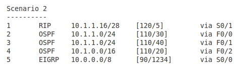
The IP packet has the destination address of 10.1.1.17. The third column on the left is the prefix learned. Which entry in the routing table (number in first column) is going to be the best in the following scenarios? Which outbound interface is going to be used?

Pic. 6 - Scenario 1.

 Pic. 7 - Scenario 2.

Pic. 8 - Scenario 3.

Pic. 9 - Scenario 4

Pic. 10 - Scenario 5

The answers to the question (all scenarios)

Scenario 1
Entry 2 is the correct answer. The egress interface is F0/0.
The router looks for the longest match in the routing table first. Entry 2 learned from RIP has the longest number of bits that are identical with the destination IP (it is the most specific). The remaining sources (OSPF and EIGRP) have fewer bits that match the destination address (they are less specific). The fact that they are more trusted does not apply here since the longest match is always preferred.

Scenario 2
Entry 1 is the correct answer. The egress interface is S0/1.
Just like in the scenario 1, the router looks for a longest match in the routing table first.
Entries 4 and 5 have 8 bits and 16 bits in common with the destination address respectively. Entries 2 and 3 have 24 bits in common. The longest match is the entry 1 having 28 networking bits that are identical with the IP address 10.1.1.17. You can check it by converting the last byte into the binary notation.

Scenario 3
Entry 2 is the correct answer. The egress interface is F0/0.
We can safely rule out the Entries 1 and 4 due to the length of network mask (not the best matches). We're left with Entries 2 and 3. Both have the same number of bits that are identical bits with the destination address (24). Both prefixes come from the same source (OSPF) and as a result of that have the same Administrative Distance value = 120. The tie breaker is going to be the metric value. Entry 2 has a cost of 30 and entry 4 has cost of 40. The lowest is the preferred one.

Scenario 4
Entry 2 is the correct answer. The egress interface is S0/0.
All five entries have the same length of prefix mask, so after longest match rule check we have five candidates.  However, entries 4 and 5 come from OSPF and have higher AD (120) than the first three entries coming from EIGRP routing protocol (90). The lower AD here is preferred. We can rule 4 and 5 out now. Again, all three of them left, have the same AD (90). The tie-breaker is the value of metric again.

Scenario 5
Entries 1 through 3 are the correct answer. The egress interfaces are S0/0, S0/1, and S0/2. The router is going to perform load balancing (traffic sharing).
We can rule out entries 4 and 5 like in the scenario 4. The remaining entries 1 through 3 come from EIGRP (AD=90) and their metrics are the same.